October 25, 2017
Home Analytics Part 1: Long Run Returns
Brodie Gay, MFE – Quantitative Strategist
In part 1 of the Home Analytics series, we will estimate a single parameter μ, the long run average return of real estate. Over a long enough timeline, the long-run historical average return of an asset provides a good first-order approximation of expected future returns.
The prior art on long-run historical average estimation is extensive. But, unlike highly homogeneous and liquid assets, each home is unique and doesn’t trade often. The estimation methods proposed herein are inspired by those methods used for more liquid asset classes but can accommodate the heterogeneity in holding periods.
Figure 1: Average long-run returns of homes. Interact with the chart to see the underlying data, data count, and standard errors. For CBSA, the bubble sizes correspond to the underlying data count.
μ̂ = 1⁄N ∑ri
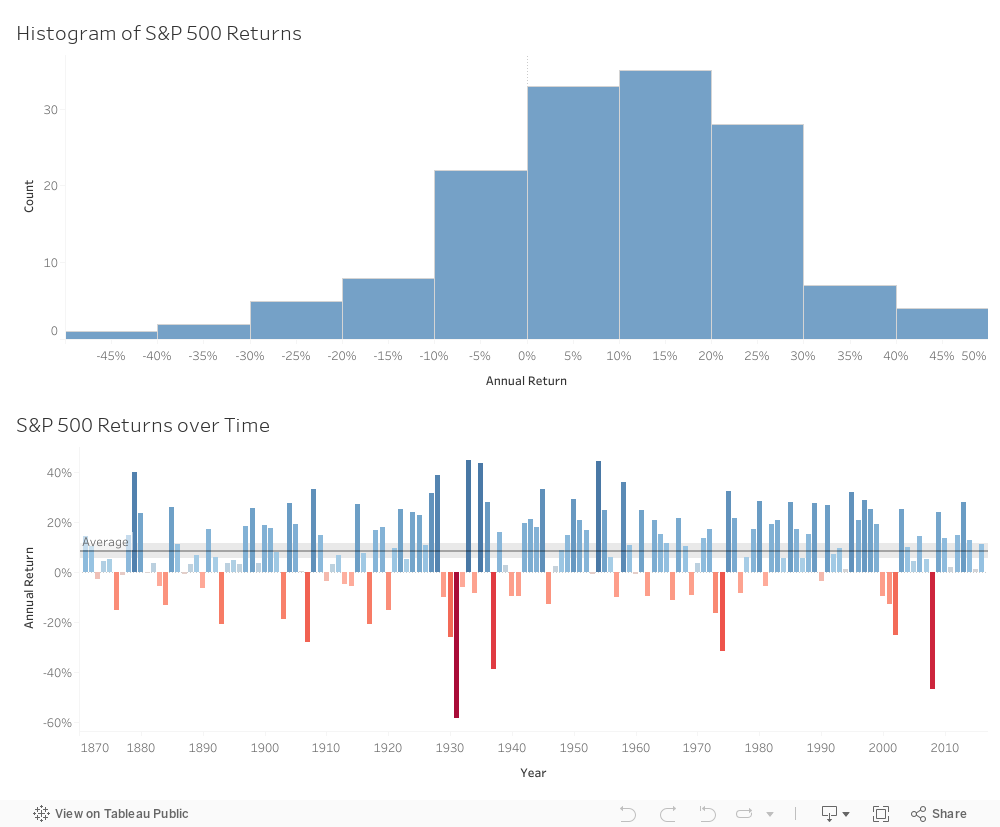
Figure 2: The last 150 years of S&P 500 total returns have returned an average of 8.7% per year Under certain assumptions, the estimate μ̂ represents the “best guess” for a return ri in the sample of assuming the following model of returns:
ri ∽ N(μ, σ2)
ri = μ + σεi
εi ∽ N(0, 1)
This return occurs over a holding period τ:
τ = T - t
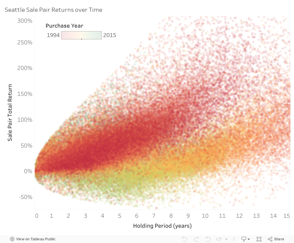
Figure 3: Observed home returns in Seattle exhibit a diffusion pattern, inspiring the use of a geometric Brownian motion model. The color coding differentiates purchase year. A small number of outliers have been removed.
If we had period-by-period returns for each home in the U.S. (e.g. a market price of each home was generated every period), the simple average formula would produce a good long-run average estimate. However, we do not control the holding period. Figure 3 suggests that both the expected return and the variance of returns increase almost linearly with the holding period. A robust model needs to adapt to the fact that both the expectation and the errors around the expectation are functions of time.
On a slightly more subtle point, despite the over 120mm homes in America, only about 20-25mm sale pairs can be generated from the past 20 years of transactions. Our model implicitly assumes that the observed returns are uniformly distributed across geography and time. This isn’t strictly true. Homes in dense urban geographies tend to outperform their rural counterparts and trade more frequently leading to a slight positive geographic bias. Separately, homes tend to turn over more quickly when the economy is strong and home price appreciation is high, leading to an additional positive temporal bias. We will explore solutions to these two sources of bias, namely geographic and temporal biases, in future posts by increasing the geographic granularity (i.e. estimating zip code level returns) and by estimating period-by-period return indices.r = ln(R + 1) = ln(psale) - ln(ppurchase)
r ∽ N(μτ, σ2τ)
This model is a simple geometric Brownian motion (GBM) diffusion model for asset returns. Buried within is an assumption that both log-returns and log-variance scale linearly with time.
E[r(τ)] = μτ
Var[r(τ)] = σ2τ
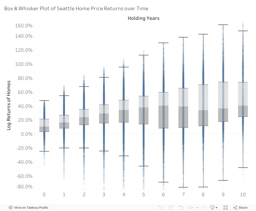
Figure 4: A box & whiskers plot of home returns shows (1) just how disperse are home returns around the average and (2) how that variance increases with time.
In future posts, we will explore the limitations of these assumptions. Some of the more important model breaks are:
For now, these assumptions only cause a slight bias in our desired estimates (and their respective standard errors).
Now that we are armed with a model of the data generating process of home returns, we can begin to think about how to estimate our parameter of interest and its standard errors.
εi ∽ N(0, 1)
We are trying to estimate μ̂ that minimizes the sum of squared errors εi2 of this model.
This beautifully simple model is both convex and has a unique closed-form solution. It is known as the weighted least-square regression:
Rewritten, the solution takes the following simplified form:
With this we can estimate the distribution, and therefore the (unbiased) standard errors, of our estimate μ̂:
Introduction
In this Home Analytics series, we will develop a toolbox of statistical methods to help analyze the home as a financial asset. We begin by estimating expected risk, returns, and correlation to other asset classes. Later, we will explore applications of our estimates as they related to the financial decisions of households, investors and the public sector. The toolbox will rely on as much historical research as possible (most notably the work of Karl Case & Robert Shiller). But, innovations will be necessary to accommodate the unique characteristics of this asset class and its data generating process.In part 1 of the Home Analytics series, we will estimate a single parameter μ, the long run average return of real estate. Over a long enough timeline, the long-run historical average return of an asset provides a good first-order approximation of expected future returns.
The prior art on long-run historical average estimation is extensive. But, unlike highly homogeneous and liquid assets, each home is unique and doesn’t trade often. The estimation methods proposed herein are inspired by those methods used for more liquid asset classes but can accommodate the heterogeneity in holding periods.
Estimated Long Run Returns
Below, we show the average historical returns for the country, states, and Core Based Statistical Areas (CBSAs), which include both larger metropolitan and smaller micropolitan areas. Included are the standard errors and data counts. The following data cleaning steps have been taken:- States and CBSAs with fewer than 10,000 sale pairs have been removed.
- Homes with more than +/-50% returns per year are removed (these are typically flips or are not arms-length transactions).
- Only homes purchased for between $50,000 and $5,000,000 are included.
- Only arms-length residential repeat sales are included (no foreclosures or short sales)
Figure 1: Average long-run returns of homes. Interact with the chart to see the underlying data, data count, and standard errors. For CBSA, the bubble sizes correspond to the underlying data count.
Inspiration for the Methodology
With the luxury of homogeneity and a dense time series of return data, a good estimate of the average long-run return μ̂ can be computed by taking the average return of the series:- μ̂ is an estimate of the long run average return
- ri is the return i in the sample of returns
Figure 2: The last 150 years of S&P 500 total returns have returned an average of 8.7% per year Under certain assumptions, the estimate μ̂ represents the “best guess” for a return ri in the sample of assuming the following model of returns:
- μ is the true long run average return
- σ2 is variance in returns
- εi is a random noise variable
.png)
.png)
Sale Pair Data
Home sales do not provide us with the same stream of period-by-period returns. In order to obtain the return for a home, we need at least two transactions: a purchase (at time t) and a sale (at time T):.png)
- Psale is the sale price
- Ppurchase is the purchase price
- R is the total holding period return
This return occurs over a holding period τ:
- T is the sale date
- t is the purchase date
- τ is the holding period
Figure 3: Observed home returns in Seattle exhibit a diffusion pattern, inspiring the use of a geometric Brownian motion model. The color coding differentiates purchase year. A small number of outliers have been removed.
If we had period-by-period returns for each home in the U.S. (e.g. a market price of each home was generated every period), the simple average formula would produce a good long-run average estimate. However, we do not control the holding period. Figure 3 suggests that both the expected return and the variance of returns increase almost linearly with the holding period. A robust model needs to adapt to the fact that both the expectation and the errors around the expectation are functions of time.
On a slightly more subtle point, despite the over 120mm homes in America, only about 20-25mm sale pairs can be generated from the past 20 years of transactions. Our model implicitly assumes that the observed returns are uniformly distributed across geography and time. This isn’t strictly true. Homes in dense urban geographies tend to outperform their rural counterparts and trade more frequently leading to a slight positive geographic bias. Separately, homes tend to turn over more quickly when the economy is strong and home price appreciation is high, leading to an additional positive temporal bias. We will explore solutions to these two sources of bias, namely geographic and temporal biases, in future posts by increasing the geographic granularity (i.e. estimating zip code level returns) and by estimating period-by-period return indices.
A Simple Model for Home Returns
Home returns tend to be log-normally distributed. Said another way, the logarithm of home returns are normally distributed. Most traded assets exhibit log-normally distributed returns r:- r is the log-return of a home
This model is a simple geometric Brownian motion (GBM) diffusion model for asset returns. Buried within is an assumption that both log-returns and log-variance scale linearly with time.
Figure 4: A box & whiskers plot of home returns shows (1) just how disperse are home returns around the average and (2) how that variance increases with time.
In future posts, we will explore the limitations of these assumptions. Some of the more important model breaks are:
- Home returns appear to be slightly auto-correlated (not independent)
- Home variance more accurately follows a jump-diffusion model, with a jump in volatility at transaction (due in part to information asymmetry/transaction costs)
For now, these assumptions only cause a slight bias in our desired estimates (and their respective standard errors).
Now that we are armed with a model of the data generating process of home returns, we can begin to think about how to estimate our parameter of interest and its standard errors.
Estimating the Long Run Average Return
Provided the following vectors of returns:
.png)
.png)
- ri is the return of sale pair i
- τi is the holding period of sale pair i
- εi is the white noise random error of sale pair i
- μ is the true long run average rate of return
- σ is the true variance rate of returns
We are trying to estimate μ̂ that minimizes the sum of squared errors εi2 of this model.
.png)
.png)
.png)
- Heterogeneity of Holding Period Returns: The prediction μτi scales with holding period
- Heterscedactic Errors: Our squared prediction errors (ri - μτi)2 are scaled by an known variance factor σ2τi
This beautifully simple model is both convex and has a unique closed-form solution. It is known as the weighted least-square regression:
.png)
.png)
Rewritten, the solution takes the following simplified form:
.png)
.png)
.png)
- σ̂2 is the maximum likelihood estimate (MLE) for return variance rate
- ŝ2 is the ordinary least square likelihood estimate (OLS) for return variance rate
With this we can estimate the distribution, and therefore the (unbiased) standard errors, of our estimate μ̂:
.png)
.png)
Conclusion
In this post, we have explored a model for long-run expected returns for homes. In the next post, we will construct a home price index. Specifically, we will describe an alternative construction of the Case-Shiller “Weighted Repeat Sales” index.Reference
Case, K.E., Shiller, R.J. (1987). Prices of single-family homes since 1970: new indexes for four citiesData
First American National Transaction Data 1996-Present.Contact UnisonIM
For more information, please contact:
Unison Investment Management
650 California Street Suite 1800 San Francisco, CA 94108
Real Estate Equity Exchange, Inc. Copyright 2023
or visit our Contact page


650 California Street San Francisco, CA 94108 | 415-992-4200 | Real Estate Equity Exchange, Inc. Copyright 2023