January 20, 2017
The Devil is in the details: risk and return in residential real estate
Executive Summary
Residential real estate equity is one of the largest asset classes in the United States and is a significant proportion of the average household’s net worth. We study how diversified real estate indices lead to a dramatic understatement of the median homeowner’s portfolio risk (by a factor of 4-5x). Finally, we explore the value of an investable and diversified residential real estate index from the perspective of an institutional investor.The Role of Residential Real Estate as an Investment
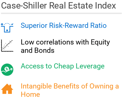
A home has some uniquely attractive investment characteristics. Using the Case-Shiller US residential home price index as a reference, the asset class has demonstrated a commanding risk-reward profile, as measured by the Sharpe ratio[1], over other conventional investments such as US equities and corporate bonds. These characteristics are summarized in Table 1.1.| Expected Return | Volatility | Sharpe | Reference | |
|---|---|---|---|---|
| U.S. Equities | 7.2% | 16.1% | 0.34 | Russell 3000 |
| Bonds | 5.8% | 9.4% | 0.43 | Barclay's U.S. Long Credit |
| Case-Shiller | 3.5% | 3.1% | 0.55 | Case-Shiller |
| Cash | 1.8% | 0.7% | n/a[2] | Treasury Bills |
Historically, the Case-Shiller index has also experienced a remarkably low correlation with stocks and bonds. Long-term capital market forecasts[3] suggest the index may experience a negative future correlation with the majority of conventional asset classes. These low correlations, shown in Table 1.2, strengthen diversification benefits.
| US Equities | Bonds | Case-Shiller | Cash | |
|---|---|---|---|---|
| U.S. Equities | 1.00 | |||
| Bonds | 0.19 | 1.00 | ||
| Case-Shiller | -0.09 | -0.04 | 1.00 | |
| Cash | 0.09 | -0.03 | -0.02 | 1.00 |
Considering that homeowners are able to borrow up to 80-90% of the value of a home at low mortgage rates, housing and portfolio returns may be amplified.
A homeowner also enjoys certain intangible benefits of living on owned property. The Panel Study of Income Dynamics[4] estimates an “imputed rent” that reflects these intangible benefits. The rent a homeowner would be willing to pay to live in their own home is approximately 4-6% of the value of the home.
Fundamentally, as populations continue to grow the demand for land and property are set to persistently outpace supply. This is especially true in urban areas.
As Figure 1.1 showcases, real estate as measured by the Case-Shiller index appears to be a very attractive investment.[3]
To demonstrate, we take the long-run expected returns, volatilities and correlations of equities, bonds, cash and the Case-Shiller index and run a portfolio optimization for various risk tolerance levels.
Figure 1.2 below represents the outcome of this analysis; illustrating the risk-reward characteristics of the following assets:
- US Equity (Russell 3000 Index)
- Bonds (Barclay’s US Long Credit Index)
- Residential Real Estate (Case-Shiller US Home Price Index)
- Cash (3 – 6 month Treasury Bill Index)
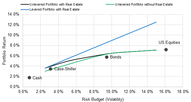
Figure 1.2 also illustrates the efficient frontier of the following three portfolios. The efficient frontiers are herein defined as the portfolio that provides the greatest expected level of return for each level of risk.
- An unlevered portfolio without residential real estate
- An unlevered portfolio with residential real estate
- A levered portfolio with residential real estate Some notable insights may be gleaned from this analysis. First, in the unlevered portfolios, higher risk investors are inclined towards US equities to achieve yield. The real estate allocation is only relevant for portfolios with a low risk tolerance. However, once leverage is permitted, the theoretically efficient portfolio invests in a mix of levered bonds with a very large real estate allocation shown in Figure 1.3.
- Asymmetric information: Buyers and sellers do not have the same information about the underlying home. Information asymmetry can be directly related to the transaction cost associated with searching for information resulting in a large bid-ask spread.
- Transaction costs: such as closing costs, real estate agent costs, and financing costs.
- Change in quality: failure of the constant quality assumption of the Case-Shiller index, which assumes that homes are all of identical quality and are not renovated or depreciated.
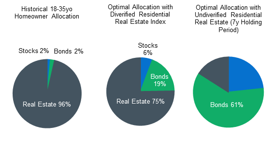
- The historical allocation of a median first time homebuyer (cash position is not shown).
- The optimal allocation provided there exists an investable diversified residential real estate index.
- The optimal allocation where the real estate component is represented by an individual home given an expected holding period of 7 years.

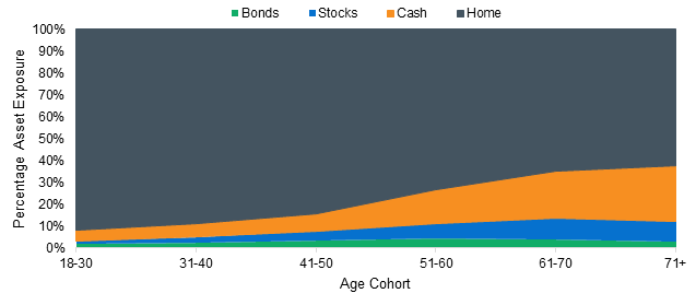
The suggested allocation for the levered portfolio is not materially different from the median household shown in Figure 1.4, which depicts the asset allocation of the average owner-occupied home.[5] The most note-worthy insight from Figure 1.4 is the magnitude of real estate exposure across all homeowner age groups.
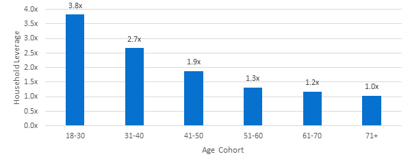
In addition to percentage allocations, the portfolio optimization results suggest a leverage of 3x the net worth of the investor for a 10% projected volatility (Figure 1.3). This is in-line with the leverage ratio of the median homeowner shown in Figure 1.5. Homeowners in this age group are risking a huge portion of their savings (up to 90%) on the down payment of a house worth 4 or 5x their net worth, respectively.
While it is acknowledged that a combination of cheap leverage, low correlations, and intangible home ownership benefits support the idea that a large real estate allocation is optimal, ultimately we argue that this conclusion is due to a widespread misunderstanding of the risks associated with real estate.
Risk of Residential Real Estate Investments, beyond the Case-Shiller Index
Thus far, we have assumed that residential real estate investments evolve with the Case-Shiller index. This is analogous to assuming that the individual stocks that make up the S&P 500 or the Russell 3000 have the same risk and return profiles of their indices. This is a very dangerous assumption. In fact, the Case-Shiller index is not an investable asset since constructing it would involve pooling small portions of equity from all of the homes in the US, which has not previously been achieved at scale.A homeowner lives in a single house. He/she is invested in a geographically-specific, heterogeneous asset. While the index is expected to only experience around 3-4% annualized volatility, it would be very unrealistic to assume that of an individual home. Figure 2.1 shows the total return distribution of every residential transaction since 1998 in the United States with a Combined Loan-to-Value (CLTV) at origination of 80-90% and a holding period of greater than one year.

Individual houses have a high degree of dispersion around the index in a given year. This dispersion tends to increase over time[6]. Additionally, there is a very short-term shock to dispersion that is apparent for exceptionally short holding periods. These shocks are quantified in the original Case-Shiller index paper and are attributed to transaction volatility jump[7] processes. If we include both this idiosyncratic volatility of the individual house as well as the short term-transaction shock, how does this affect the portfolio of our average homeowners?
Components of Risk and the Effect on the Homeowner Portfolio:
Under the Case-Shiller model, the price of a house generally follows the following process:
(a) Systemic Index Risk (β):
The risk we are most familiar with is the market-wide Case-Shiller risk. This risk has the unique feature that it cannot be diversified away, whereas the idiosyncratic and transactional shocks would disappear in a large portfolio of real estate.
This risk is largely associated with the volatility of the Cash-Shiller Home Price Index. Unlike other popular indices, the Case-Shiller index is not investable and, as a result, not particularly useful for portfolio construction. By including the idiosyncratic component of a home, we can begin to make realistic predictions about the performance of a homeowner’s portfolio
(b) Idiosyncratic Risk (H):
The Case-Shiller Home Price Index paints a very optimistic picture for residential real estate as an investment vehicle. But it has been long known to fail in its representation of a homeowners’ experience, especially during turbulence of the last decade. First, it fails to appreciate the fact that an individual home does not simply follow the average index. In fact, the average home has a significant idiosyncratic component.
Case and Shiller, in their foundational paper on the weighted-repeat sales methodology, which is the basis for the Case-Shiller model, quantify this idiosyncratic component, estimating it to be around 7% for San Francisco (in the period 1970-1986). Using our transaction dataset for the period 1996-2016, we have estimate it to be ~10% nationwide.[8]
Many research articles try to revise portfolio optimization problems by including this idiosyncratic component of risk when crafting the homeowner portfolio. In particular, Flavin and Yamashita (2002) borrow the total volatility estimate (Index Volatility + Idiosyncratic Volatility) from the Panel Study of Income Dynamics. In addition to adding the idiosyncratic risk component, they also add a return premium to real estate to compensate for the imputed rent and treat the real estate position as a constraint on a portfolio rather than a highly divisible asset (such as stocks and bonds). Most importantly, though, is their conclusion that a single home is significantly riskier than previously assumed. Even the imputed rent premium cannot compensate an investor/homeowner enough to validate taking such a levered and risky position.
One risk that has yet to be included in the portfolio optimization exercise is the jump process associated with transaction shocks, even though this risk was identified several decades ago.
(c) Transaction Shocks (N):
Case and Shiller highlight a separate risk that is independent of holding period. Specifically, their study shows that there is stochastic jump in price that occurs as a result of the transaction of these large illiquid assets. There are various theories associated with this risk source:
Case and Shiller estimate this transaction noise at around 7% of volatility per transaction, whereas in more recent years we estimate it to be up to 15% of volatility per transaction in some geographies[9].
Table 3.1 summarizes the decomposition of real estate price appreciation. In addition, we provide an analogy of each component to the equity markets.
| Component | Real Estate | Risk (volatility) | Equity | Risk (volatility) |
|---|---|---|---|---|
| Index Risk | Case-Shiller Home Price Index | 3-4% per year | Russell 3000 | 16% per year |
| Idiosyncratic Risk | Individual Home in SF | 7-10% per year | Individual Stock AAPL | 20% per year |
| Transaction Noise | Sale of Home in SF | 7-15% per transaction | AAPL Bid/Ask Spread | 1bp per transaction |
| Cash | 0.09 | -0.03 | -0.02 | 1.00 |
Figure 3.1 shows how the risk (volatility) evolves over holding period for the 4 common assets.
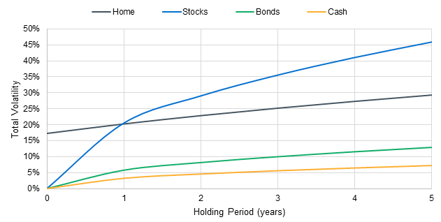
Note that unlike highly liquid and homogeneous assets like stocks, bonds, and cash (T-bills), the homeowner experiences volatility of real estate even if the holding period is as short as a few days. This is a result of two independent jump processes associated with purchasing and selling the home. Notably, while real estate is often considered to be a low-risk investment vehicle, this is only strictly true over a long holding period. Therefore, liquidity shocks that force a homeowner to sell can have devastating effects on a portfolio due to the price-jump risk at sale paired with the large amount of leverage that will get called due when the sale occurs.
Figure 3.2 shows how the risk of the first-time homebuyer (18-30 age cohort) amplifies under realistic assumptions about volatility of the asset.
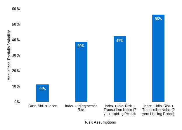
To put things into perspective, this portfolio would be the equivalent of investing one’s entire wealth into an individual stock such as Netflix, Amazon, or Tesla. We also note that the holding period has a significant effect on the volatility of the portfolio. The difference between a two year holding period and the average seven year holding period of a home can result in a 25% increase in volatility.
Returning to the portfolio optimization exercise, Figure 3.3a shows the 3 portfolio allocations:
In Figure 3.3b, we show the efficient frontier of the two optimal portfolios introduced above as well as the risk-return profile of the 18- 35-year-old homeowner.
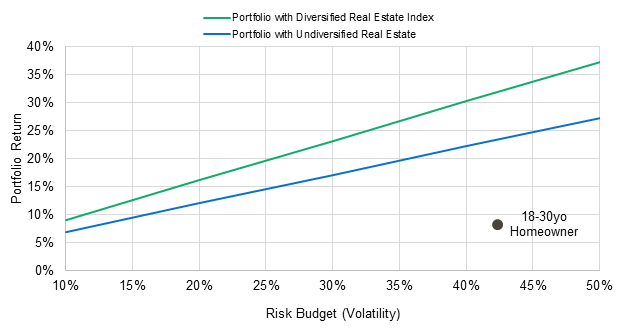
Figure 3.3b shows the homeowner is both taking on an incredible amount of risk and isn’t being rewarded for it. The homeowner’s portfolio would be made significantly more efficient by rotating out of residential real estate equity into bonds and stock (right-most chart in Figure 3.3a).
Separately, a diversified real estate portfolio without the idiosyncratic risk and transaction noise components of a single home extends the efficient investment frontier by a noteworthy amount. The optimal allocation when an investable, diversified real estate index is provided suggests that there would be a large institutional demand for such an asset class if it existed.
Conclusion
On a national scale, housing is an incredibly efficient investment. However, while homes in the US tend to appreciate, on average, consistently each year, as it stands, tens of trillions of dollars of home equity are currently being held in separate, individually undiversified, and heavily levered portfolios. This means that every year, many homeowners have incredible windfalls while others are forced to declare bankruptcy or have their houses foreclosed on.
When assuming that the price of a home perfectly follows the Case-Shiller index, the portfolio of a young homeowner comprising 3x leverage and almost 90% exposure to residential real estate is actually quite well supported by modern portfolio theory, especially when the intangible benefits of owning a home are considered. However, when more realistic assumptions about the risk of an individual home are included, the overall volatility of such an exposed portfolio increases up to 4-5 times, with no commensurate increase in expected return.
This conclusion suggests that homeowner financing should be fundamentally rethought. First, we must note the incredible value of the successful construction of a residential real estate index. The majority of real estate risk is idiosyncratic in nature and can therefore be diversified away at the portfolio level. Secondly, we should explore new ways of financing home purchases beyond mortgage instruments. A risk averse investor would benefit greatly from the ability to sell equity rather than just debt in their home. By selling equity, they can reduce their exposure to the risky home and allocate it toward a more diverse allocation of assets.
Research References:
Case, Karl E. and Robert J Shiller. 1987. “Prices of single family homes since 1970: new indexes for four cities” National Bureau of Economic Research.
Flavin, Marjorie and Takashi Yamashita. 2002. “Owner-Occupied Housing and the Composition of the Household Portfolio” American Economic Review.Data References:
BNY Mellon Long-Term Capital Market Report 2016
First American Property and Transaction Level Data
Panel Study of Income Dynamics (https://psidonline.isr.umich.edu/)Footnotes:
[1] The Sharpe ratio is defined as the expected return of an asset (in excess of the risk-free or cash rate of return) divided by the expected volatility of the rate of return.
[2] Sharpe Ratios are calculated in excess of the cash position.
[3] Long-term capital market forecasts are taken from the BNY Mellon Long-Term Capital Market Report 2016.
[4] The PSID measures economic factors over the entire life cycle of families, for multiple generations.
[5] Flavin and Yamashita (2002).
[6] A diffusion process is one in which variance (the square of volatility) increases linearly with time. This is a common feature of assets that follow a Brownian diffusion process like stocks and bonds.
[7] A jump process represents a sudden volatility shock that is independent of time. A process with both diffusion and jump processes is known as a jump-diffusion process.
[8] Using nationwide sale pair data provided by First American, we applied a weighted repeat sales method for the period ranging between 1996-2016
[9] We estimated the holding period structure of the idiosyncratic risk using the Case-Shiller Weighted Repeat Sales approach on single family home sale pairs data supplied by First American©.
Contact UnisonIM
For more information, please contact:
Unison Investment Management
4 Embarcadero Center, Ste. 710, San Francisco, CA 94111
Real Estate Equity Exchange, Inc. Copyright 2023
or visit our Contact page


©2025 Unison Investment Management, LLC | 4 Embarcadero Center, Ste. 710, San Francisco, CA 94111 | 415-992-4200